Sample code fragments for creating commonly used exhibits in empirical research projects.

Two-sample t-test of multiple variables

Table (estout/esttab)

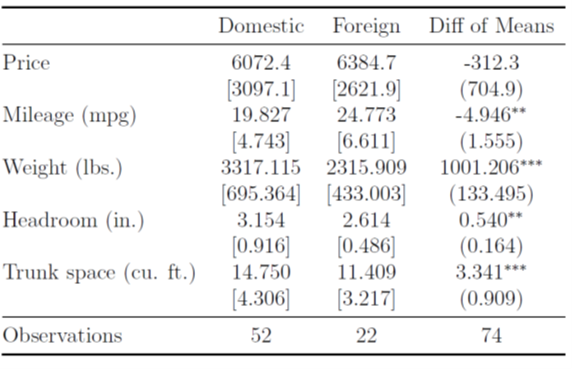
Stata code

sysuse auto, clear

** Formatted table in LaTeX
eststo clear
eststo domestic: estpost tabstat price mpg weight headroom trunk if foreign == 0, columns(statistics) statistics(count mean sd p25 p50 p75)
eststo foreign: estpost tabstat price mpg weight headroom trunk if foreign == 1, columns(statistics) statistics(count mean sd p25 p50 p75)
eststo diff: estpost ttest price mpg weight headroom trunk, by(foreign) unequal
esttab domestic foreign diff using two_sample_ttest.tex, ///
    cells("mean(pattern(1 1 0) f(1 3))  b(star pattern(0 0 1) f(1 3))" "sd(par([ ]) f(1 3) pattern(1 1 0)) se(pattern(0 0 1) par f(1 3))") ///
    label mlabels("Domestic" "Foreign" "Diff of Means") substitute(% \%) collabels(,none) ///
    prehead(`"\def\sym#1{\ifmmode^{#1}\else\(^{#1}\)\fi}"'  \begin{tabular}{@{\extracolsep{\fill}}l*{@E}{c}} \toprule ) ///
    postfoot(`"\bottomrule"' \end{tabular}) nonotes replace booktabs noisily compress nonum

[Download the Stata code] Note: The code for the same table in different format is included in the do file.

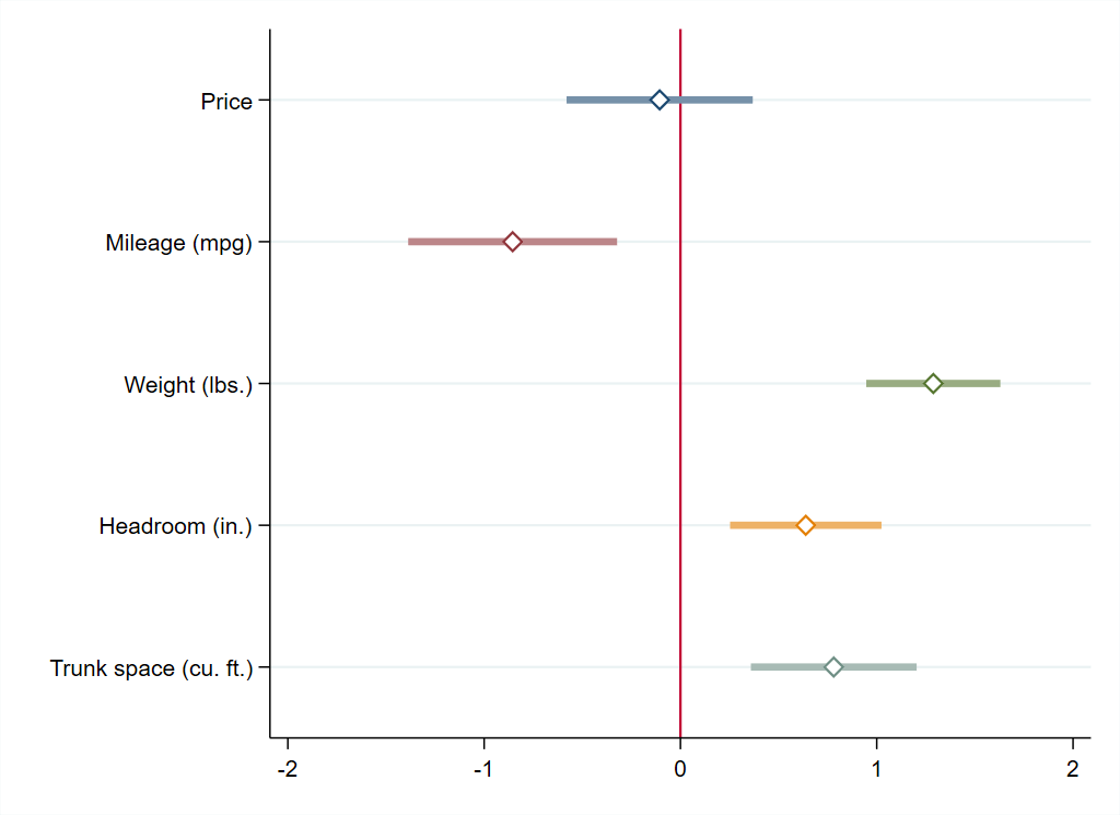
Figure (estout/esttab, coefplot)

If the scale is similar across variables, the t-test result can be graphically presented. The scale varies a lot in the auto dataset. For illustration purposes, I create the figure using standardized versions of these variables.

Stata code

sysuse auto, clear
foreach var in price mpg weight headroom trunk {
    egen `var'_z = std(`var')
    _crcslbl `var'_z `var'
}

estpost ttest price_z mpg_z weight_z headroom_z trunk_z, by(foreign) unequal

recode foreign (0=1) (1=0)
foreach var in price mpg weight headroom trunk {
    gen `var'_2 = foreign
    _crcslbl `var'_2 `var'
    quietly regress `var'_z `var'_2, robust
    estimates store `var'
}

coefplot price mpg weight headroom trunk ///
    , drop(_cons) nooffsets xline(0) xlabel(, labsize(small)) msymbol(D) mfcolor(white) ciopts(lwidth(*3) lcolor(*.6)) ///
    ylabel(,labsize(small) glcolor(gs7) glwidth(vvthin)) graphregion(color(white)) legend(off)
graph export "ttest_figure.png", as(png) width(1024) replace

[Download the Stata code]